Adiabatic theory of strong-field ionization of molecules including nuclear motion

Jens Svensmark

January 21, 2020

My background

Aarhus University

PhD

Kansas state university

Postdoc

University of Electro-communications (Tokyo)

Postdoc

Intro

Adiabatic theory

Previously been used for atoms
Here we look at molecules

Time scales

Laser
Motion inside molecule
Ratio is adiabatic parameter

Adiabatic approximation

Adiabatic parameter small
Laser field momentarily constant
Sequence of stationary Siegert states

Sequence of stationary states

Previous work

Looked at atoms/fixed nuclei
Electrons are fast
Laser is slow
How about nuclei?

PRA 86, 043417 (2012)

PRA 92, 043402 (2015)

PRL 116, 173001 (2016)

What we want to do

Extend adiabatic theory to molecules including nuclear motion

Numerical calculations

1D model

Time-dependent Schrödinger equation

\begin{align} i\frac{\partial }{\partial t} \Psi(x,R,t) & = [H_0+F(t) x] \Psi(x,R,t) \end{align}

\begin{align} H_0 = -\frac{1}{2m}\frac{\partial^2}{\partial x^2}-\frac{1}{2\mu} \frac{\partial^2}{\partial R^2} + V(x;R)+U_\text{ion}(R) \end{align}

Numerical methods

Split step fourier method

Scattering states found using R-matrix propagation

Fixed nuclei example

Adiabatic theory (fixed nuclei)

\(\epsilon = \frac{T_\text{e}}{T_\text{f}} \to 0\)

Photo electron momentum distribution (PEMD)

\begin{align} P(k) & = \frac{2\pi}{\left| F(t_i) \right|} \left| f(F(t_i)) \right|^2 e^{- \int_{-\infty}^{t_i} \Gamma(F(t)) dt} \end{align}

\(k:\) Momentum of outgoing electron

\(t_i\) is time at which electron with momentum \(k\) ionized, \(k = -\int_{t_i}^{\infty} F(t')dt'\)

Pulse

Adiabatic theory (fixed nuclei)

\(\epsilon = \frac{T_\text{e}}{T_\text{f}} \to 0\)

Photo electron momentum distribution (PEMD)

\begin{align} P(k) & = \frac{2\pi}{\left| F(t_i) \right|} \left| f(F(t_i)) \right|^2 e^{- \int_{-\infty}^{t_i} \Gamma(F(t)) dt} \end{align}

\(k:\) Momentum of outgoing electron

\(t_i\) is time at which electron with momentum \(k\) ionized, \(k = -\int_{t_i}^{\infty} F(t')dt'\)

\(f(F), \Gamma(F):\) Properties of Siegert state

Siegert state

Solution of time independent Schrödinger equation

\begin{align} [H_0 + Fx] \Phi(x, R; F) & = E(F) \Phi(x, R; F) \end{align}

with outgoing-wave boundary conditions.

Outgoing wave

Adiabatic theory (fixed nuclei)

Photo electron momentum distribution (PEMD)

\begin{align} P(k) & = \frac{2\pi}{\left| F(t_i) \right|} \left| f(F(t_i)) \right|^2 e^{- \int_{-\infty}^{t_i} \Gamma(F(t)) dt} \end{align}

\(k:\) Momentum of outgoing electron

\(t_i\) is time at which electron with momentum \(k\) ionized, \(k = -\int_{t_i}^{\infty} F(t')dt'\)

\(f(F):\) Asymptotic wave function coefficient

\(\Gamma(F):\) Total rate

Weak field limit

For \(F\to 0\) adiabatic theory reduces to Keldysh theory

Nuclear-electron interaction

\begin{align} V(x; R) = V\left(x+\frac{1}{2}R\right) + V\left(x-\frac{1}{2}R\right) \end{align}

Finite range potential

\begin{align} V(x)&=-\frac{a}{\cosh^2(bx)}, \end{align}

with \(a = 0.62772\) and \(b = 0.857\).

Gaussian half-cycle pulse

\begin{align} F(t) & = F_0\exp\left(-\left[\frac{2t}{T}\right]^2\right) \end{align}

TDSE solution

Convergence to adiabatic theory

Including nuclear motion

Nuclear-nuclear interaction

H\(_2^+\) like interaction

\begin{align} U_\text{ion}(R) & = \frac{A}{R^2} + B + C R^2 \end{align}

with \(A=0.26, B =-0.732635\) and \(C =0.01625\)

\(R\) is the internuclear seperation

Vibrational states, molecular ion

\begin{align*} \left[-\frac{1}{2\mu} \frac{d^2}{dR^2} + U_\text{ion}(R)\right] \chi_v(R) = \varepsilon_v \chi_v(R) \end{align*}

Adiabatic theory

\(\epsilon_\text{f} = \max\left(\frac{T_\text{e}}{T_\text{f}}, \frac{T_\text{n}}{T_\text{f}}\right) \to 0\)

PEMD (for half-cycle pulse)

\begin{align*} P_v(k) & = \frac{2\pi}{m^2} \frac{|f_{v}(F(t_i))|^2}{ |F(t_i)|} e^{-\int_{-\infty}^{t_i} \Gamma(F(t')) dt'} \end{align*}

Total PEMD

\begin{align*} P(k) = \sum_v P_v(k) \end{align*}

Siegert state (real part)

PEMD

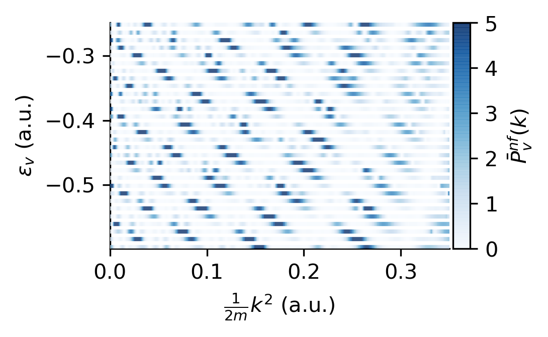
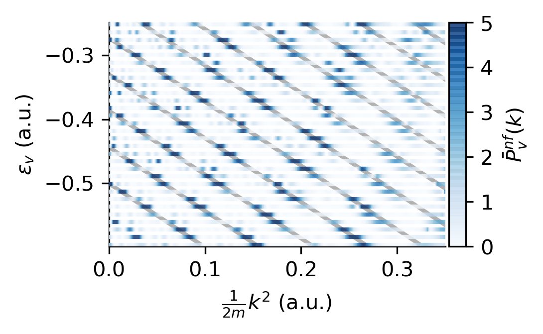
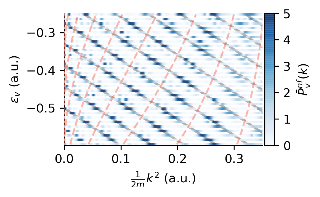
Slow nuclei and field (AAnf)

AAnf

\(\epsilon_\text{nf} = \max\left(\frac{T_\text{e}}{T_\text{f}}, \frac{T_\text{e}}{T_\text{n}}\right) \to 0\)

Born-Oppenheimer ansatz

\begin{align*} \Psi_{\text{BO}}(x,R,t) = \Psi(R, t)\psi_e(x;R,F(t)) \end{align*}

Electronic Siegert state \(\psi_e(x;R,F(t))\)

\begin{align*} \left[H_x(F) - E_e(R,F)\right] \psi_e(x;R,F) = 0 \end{align*}

where

\(H_x(F) = -\frac{1}{2}\frac{\partial^2}{\partial x^2} + Fx + V\left(x; R\right)\)

AAnf

Born-Oppenheimer ansatz

\begin{align*} \Psi_{\text{BO}}(x,R,t) = \Psi(R, t)\psi_e(x;R,F(t)) \end{align*}

Nuclear wavefunction fulfills

\begin{align*} i\frac{\partial}{\partial t}\Psi(R, t) & = \left[-\frac{1}{2\mu} \frac{\partial^2}{\partial R^2} + E_e(R,F(t))\right] \Psi(R, t) \end{align*}

Nuclear time evolution

PEMD

\begin{align*} P_v^{\text{AAnf}}(k) & = \frac{2\pi }{|F(t_i)|} \left| g_v(t_i) \right|^2 \\ \end{align*}

\begin{align*} g_v(t) = \int_0^\infty \chi_v (R) f(R,F(t)) \Psi(R,t) dR, \end{align*}

\begin{align*} \psi_e(x;R,F)|_{|x|\to \infty} = f(R,F) f(x,E_e(R,F),F) \end{align*}

Build the PEMD

PEMD

Regions of applicability

AAf

\begin{align*} \epsilon_\text{f} = \max\left(\frac{T_\text{e}}{T_\text{f}}, \frac{T_\text{n}}{T_\text{f}}\right) \to 0 \end{align*}

AAnf

\begin{align*} \epsilon_\text{nf} = \max\left(\frac{T_\text{e}}{T_\text{f}}, \frac{T_\text{e}}{T_\text{n}}\right) \to 0 \end{align*}

Regions of applicability

Compatibility

Small nuclear masses

\(T=30\) a.u.

Small nuclear masses

\(T=150\) a.u.

Few-cycle pulse

Pulse

\begin{align*} P_v^{\text{AAnf}}(k) & = \left|\sum_i \frac{\sqrt{2\pi} e^{i\pi/4} }{\sqrt{s_i F(t_i)}} e^{i\mathcal{S}_a(t_i,v; k)} g_v(t_i) \right|^2 \end{align*}

Build the PEMD

PEMD

Closer look at the nuclear wave function

Nuclear time evolution

Classical trajectory

Many-cycle pulse

How much time does TDSE take?

PEMD

Many-cycle model

\begin{align} F(t) = F_0 \cos \omega t \end{align}

\begin{align} P_{v}^{\text{AAnf}}(k) \propto % 2\pi \frac{\left|\tilde{g}_{v}(t_{(0, 1)})\right|^2}{\left|F(t_{(0, 1)})\right|} \left|p^{\text{inter}}(k)\right|^2 \left|p^{\text{intra}}(k)\right|^2 \end{align}

Similar to SFA based model in PRA 93, 031401

Inter-cycle factor

\begin{align} \left|p^{\text{inter}}(k)\right|^2 = e^{-c(k)} \left|\frac{\sin^2 [N d(k)]}{\sin^2 d(k)}\right| \end{align}

\begin{align} d(k) & = \pi \omega^{-1} \Delta E(k) \color{gray} { + \frac{1}{2}s_0^{\text{cycle}}}\\ \Delta E(k) & = E_0^{\text{BO}}-\varepsilon_v - \frac{1}{2 m} k^2 - U_p \end{align}

Ponderomotive energy: \(U_p = \frac{F_0^2}{4m\omega^2}\)

PEMD

Intra-cycle factor

\begin{align} p^{\text{intra}}(k) = 2 \cos \frac{\Delta\mathcal{S}_a(k)}{2} \end{align}

\begin{align} \Delta \mathcal{S}_a(k) = & - \omega^{-1} \Delta E(k) \left[-2\sin^{-1} \frac{k\omega}{F_0}+\text{sgn}(k) \pi\right] \\ & - \frac{3}{2}k \frac{F_0}{m\omega^2} \sqrt{1 - \left(\frac{k\omega}{F_0}\right)^2}- \Delta s_0 \end{align}

PEMD

Recap

Goal: Extend adiabatic theory
AAf only works for small nuclear masses in slow fields
AAnf works for large nuclear masses in slow fields
Possible next: include rescattering
Possible next: include dissociation

Deleted scenes

Introduction

Breakdown of BOA

What we want to look at

BOA breaks down in weak-field limit for total rate
WFAT gives total rate
Adiabatic theory gives differential quantities
Differential quantities might show other BO-breakdowns

Numerical calculations

Time-independent Schrödinger equation

Scattering boundary conditions

\begin{align} H_0 \Psi(x,R) & = E \Psi(x,R) \end{align}

Boundary conditions

\begin{align} \Psi_-^{\text{out}}(x,k) & = \begin{cases} e^{-ikx} - r^* e^{ikx} & x\leq x_-\\ t^* e^{-ikx} & x\geq x_+ \end{cases} \end{align}

\(\Psi_+^{\text{out}}(x,k)\)

Scattering solution method

R-matrix propagation in \(x\)
Adiabatic basis in \(R\) for fixed \(x\)
Sectorized legendre DVR in \(x\)
Sine-DVR in \(R\)

Different grids

One cycle pulse

Pulse

\begin{align*} P_v^{\text{AAnf}}(k) & = \left|\sum_i \frac{\sqrt{2\pi} e^{i\pi/4} }{\sqrt{s_i qF(t_i)}} e^{i\mathcal{S}_a(t_i,v; k)} R_v(t_i) \right|^2 \end{align*}

Build the PEMD

\begin{align*} P_v^{\text{AAnf}}(k) & = \left|\sum_i \frac{\sqrt{2\pi} e^{i\pi/4} }{\sqrt{s_i F(t_i)}} e^{i\mathcal{S}_a(t_i,v; k)} R_v(t_i) \right|^2 \end{align*}